Table of Contents
Tutorial 3: Balanced network with synaptic plasticity (triplet STDP)
Here you will learn to extend the balanced network model we hacked together in Tutorial 2 with plastic synapses.
As you have seen in the previous section the firing rate distribution is relatively wide in our random network. Moreover firing rates are pretty high. If you have tried to tune the weights such that the network exhibits a more plausible activity level, you might have noticed that this not completely trivial and the rates can in fact be quite sensitive to the synaptic weight parameters.
However, we know that real synapses are plastic and a diversity of plasticity processes is at work in real neural networks which could achieve this tuning automatically. Let's now extend our previous model with one form of homeostatic plasticity. To that end we would like to exchange our sparse static connectivity of the excitatory-to-excitatory synapses in Tutorial 2 with plastic synapses. Here we will use a homeostatic form of Triplet STDP with a rapid sliding threshold (see this article for more details on why it needs to be rapid).
The code of this example can be found here https://github.com/fzenke/auryn/blob/master/examples/sim_tutorial3.cpp
Changing the static model to a plastic model
All we need to change in our previous code is to replace the line in which we define con_ee with the following code
float tau_hom = 5.0; // timescale of homeostatic sliding threshold
float eta_rel = 0.1; // relative learning rate
float kappa = 3.0;   // target rate
TripletConnection * con_ee = new TripletConnection(neurons_exc,neurons_exc,weight,sparseness,tau_hom,eta_rel,kappa);
con_ee->set_transmitter(GLUT);
con_ee->stdp_active = false;
where as you can see we used TripletConnection instead of SparseConnection and we defined some additional parameters that you can play with later. Moreover we disable STDP for now so the homeostatic rate detector which controls the amount of LTD in the triplet STDP model can first adjust itself. We will turn plasticity on after an initial burn in period.
Adding a population rate monitor
To see what plasticity does it is also convenient to monitor the population rates over time. Instead of computing this off-line we can efficiently monitor it on-line with a PopulationRateMonitor.
Let's add that below the monitors that we defined previously:
PopulationRateMonitor * prate_mon_exc = new PopulationRateMonitor(neurons_exc, sys->fn("exc","prate"));
PopulationRateMonitor * prate_mon_inh = new PopulationRateMonitor(neurons_inh, sys->fn("inh","prate"));
Running the simulation
Now it's time to schedule our run. Remember we want to simulate the network for an initial burn in period, say 10s, and then activate STDP. After that we would like to continue the simulation. Let's do that:
// Run the simulation for 10 seconds
sys->run(10);
// Run the simulation for 100 seconds
con_ee->stdp_active = true;
sys->run(100);
That's it. Save the file and let's compile and run!
Speeding up simulations: Parallel execution with MPI
By now you have simulated plastic recurrent spiking neural networks with Auryn. You might have noticed that these simulations have started to be increasingly time consuming. Fortunately, most code can be sped up considerable by running simulations in parallel. This can be done transparently in Auryn. Learn how it's done here.
Visualizations
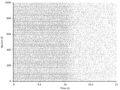
As you can see the transition around 10s where we switch plasticity on is quite drastic:

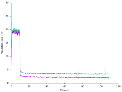
To appreciate this in more detail, let us take a look at the new files from the population rate monitors with the extension prate. We can directly plot those files as time series:

As we can see the transition to low firing rates is indeed quite rapid, but the target rate of kappa = 1.0 is not achieved during the simulation time frame. Note also the synchrony events around t=~75s and t=~105s where the network briefly leaves the asynchronous state.
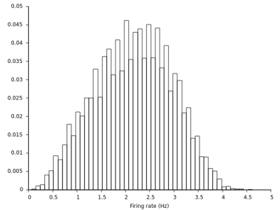
Finally we can look at the firing rate distribution of homeostatic triplet STDP (every neuron in the model has the same homeostatic target rate, so we expect something uni-modal).

Exercises
- Speed up the simulation using parallelism
- Find a slower tau for which the network activity oscillates or explodes (see for details)
- Add inhibitory synaptic plasticity to this simulation (see SymmetricSTDPConnection)
