Here you will learn to simulate a single AdEx neuron and record spikes and membrane potentials.

First create a new file named sim_mysolution1.cpp and make it a regular C++ program:

int main(int ac, char* av[])
{
 
}

To make this an Auryn simulation all we need to do is to import its header file and call the following functions which prepare the Auryn kernel and set some global variables.

#include "auryn.h"
using namespace auryn;
int main(int ac, char* av[])
{
  auryn_init( ac, av );
 
  // the simulation code will go here
 
  auryn_free();
}

For convenience we also set our current namespace to Auryn's namespace. You also might want to specify an output directory, a simulation name and maybe the name of the logfile. All these information can be passed as additional parameters to auryn_init. This hasn't been done here for simplicity.

You can now compile this program and run it, but it won't do anything other than writing a log file.

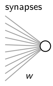
To actually have your simulation do something, we want to build the following network model: in which a single AdEx neuron receives input from 100 Poisson neurons. We will do this in three steps. First, we define all the populations of neurons which generate or receive spikes. Second, we will connect these classes with synaptic connections. Finally, we will define some special classes which will allow us to readout information from the simulation and store it to disk.

Populations in Auryn are abstracted as SpikingGroup or NeuronGroups. Let's first set up our input. We want 100 Poisson neurons which should fire at 5Hz. After auryn_init we write

int nb_input_neurons = 100;
float poisson_rate = 5.0;
PoissonGroup * poisson = new PoissonGroup(nb_input_neurons,poisson_rate);

We now have a PoissonGroup in our simulation. Now we need the one AdEx neuron we wanted to simulate. This we get by adding the following line (all before auryn_free which ends the simulation code).

AdExGroup * neuron = new AdExGroup(1);

Here the “1” sais that we want only one neuron in the group. For network simulations you will typically have more than one. You would write 2000 or whatever number of neurons you want.

Now we need to connect the input with our AdEx neuron. For this simple example we choose all-to-all connectivity:

float weight = 0.2; // conductance amplitude in units of leak conductance
AllToAllConnection * con = new AllToAllConnection(poisson, neuron, weight);

This is an excitatory connection by default, but let's make this clear in the code by adding the following line:

con->set_transmitter(GLUT);

You could have written GABA to make this a GABAergic connection instead.

Now we are almost done setting up our model, but the simulation would still run without producing any output. Let's say we want to record the input and output spikes and the postsynaptic voltage. This is how we rig our Monitors.

SpikeMonitor * input_spike_mon = new SpikeMonitor( poisson, sys->fn("input","ras") );
SpikeMonitor * output_spike_mon = new SpikeMonitor( neuron, sys->fn("output","ras") );
VoltageMonitor * output_voltage_mon = new VoltageMonitor( neuron, 0, sys->fn("output","mem") );

The last arguments for each of those is the filename where we want to write the output. The fn function provided by sys returns a file name and makes it parallel save (which will become important later).

One comment is in order: Writing output to disk is computationally expensive. It's often possible to speed up a simulation substantially by reducing the amount of data that's saved. Choose the variables you want to record carefully and you will be rewarded with code that runs much faster.

Now all that's left to do is to tell the Auryn kernel how long we want to run our simulation. Let's say we want to run for 2 seconds. We write:

sys->run(2);

where sys is the global pointer variable pointing to the Auryn kernel (which was initialized by auryn_init(ac,av) above).

That's it! Now we can compile and run the simulation. Note, in my example I had named the file sim_tutorial1, but you have chosen a different name.

$ make && ./sim_tutorial1
$ [=========================] 100%      t=2.0s  f=5.9 Hz in SpikingGroup
$ ls -ltrs | tail -n 5
  860 -rwxrwxr-x  1 zenke zenke   878792 Sep  1 11:48 sim_tutorial1
    4 -rw-rw-r--  1 zenke zenke      981 Sep  1 12:12 sim_tutorial1.0.log
    4 -rw-rw-r--  1 zenke zenke      462 Sep  1 12:12 output.0.ras
  372 -rw-rw-r--  1 zenke zenke   379984 Sep  1 12:12 output.0.mem
   12 -rw-rw-r--  1 zenke zenke    12002 Sep  1 12:12 input.0.ras

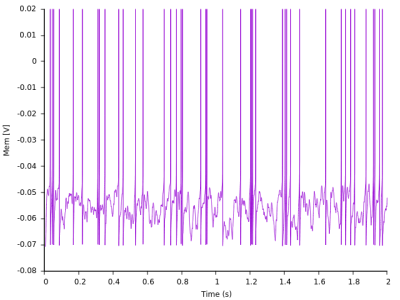
Each monitor has written its own output file. Let's take a look at the membrane potential, which is the file with the mem extension.

I like plotting things in gnuplot, but you might have your own preferences such as Python matplotlib or something else. The ras and mem files are human readable ASCII files (you can just open them with an editor to see their structure) so most plotters should work.

Here is my voltage trace as plotted by Gnuplot:

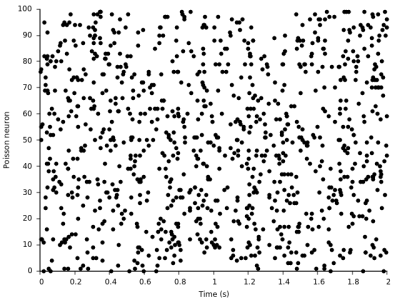
And here are the input Poisson spikes

You find the code of this simulation under examples/sim_tutorial1.cpp https://github.com/fzenke/auryn/blob/master/examples/sim_tutorial1.cpp

In the next section you will learn how to simulate a recurrent network model instead of single neuron.

• Play with different rate values for the Poisson processes
• Replace the AdEx by an Izhikevich neuron
• Add a second Poisson input population which provides inhibitory input to the output neuron
• Simulate 2 or more neurons and connect them with sparse connectivity (see SparseConnection). Then visualize the different voltage traces (note that you will have to define a different VoltageMonitor instance for each neuron you record from).